4. Attention Mechanisms
Attention Mechanisms and Self-Attention in Neural Networks
Attention mechanisms allow neural networks to focus on specific parts of the input when generating each part of the output. They assign different weights to different inputs, helping the model decide which inputs are most relevant to the task at hand. This is crucial in tasks like machine translation, where understanding the context of the entire sentence is necessary for accurate translation.
[!TIP] The goal of this fourth phase is very simple: Apply some attetion mechanisms. These are going to be a lot of repeated layers that are going to capture the relation of a word in the vocabulary with its neighbours in the current sentence being used to train the LLM.\ A lot of layers are used for this, so a lot of trainable parameters are going to be capturing this information.
Understanding Attention Mechanisms
In traditional sequence-to-sequence models used for language translation, the model encodes an input sequence into a fixed-size context vector. However, this approach struggles with long sentences because the fixed-size context vector may not capture all necessary information. Attention mechanisms address this limitation by allowing the model to consider all input tokens when generating each output token.
Example: Machine Translation
Consider translating the German sentence "Kannst du mir helfen diesen Satz zu übersetzen" into English. A word-by-word translation would not produce a grammatically correct English sentence due to differences in grammatical structures between languages. An attention mechanism enables the model to focus on relevant parts of the input sentence when generating each word of the output sentence, leading to a more accurate and coherent translation.
Introduction to Self-Attention
Self-attention, or intra-attention, is a mechanism where attention is applied within a single sequence to compute a representation of that sequence. It allows each token in the sequence to attend to all other tokens, helping the model capture dependencies between tokens regardless of their distance in the sequence.
Key Concepts
- Tokens: Individual elements of the input sequence (e.g., words in a sentence).
- Embeddings: Vector representations of tokens, capturing semantic information.
- Attention Weights: Values that determine the importance of each token relative to others.
Calculating Attention Weights: A Step-by-Step Example
Let's consider the sentence "Hello shiny sun!" and represent each word with a 3-dimensional embedding:
- Hello:
[0.34, 0.22, 0.54] - shiny:
[0.53, 0.34, 0.98] - sun:
[0.29, 0.54, 0.93]
Our goal is to compute the context vector for the word "shiny" using self-attention.
Step 1: Compute Attention Scores
[!TIP] Just multiply each dimension value of the query with the relevant one of each token and add the results. You get 1 value per pair of tokens.
For each word in the sentence, compute the attention score with respect to "shiny" by calculating the dot product of their embeddings.
Attention Score between "Hello" and "shiny"

Attention Score between "shiny" and "shiny"

Attention Score between "sun" and "shiny"

Step 2: Normalize Attention Scores to Obtain Attention Weights
[!TIP] Don't get lost in the mathematical terms, the goal of this function is simple, normalize all the weights so they sum 1 in total.
Moreover, softmax function is used because it accentuates differences due to the exponential part, making easier to detect useful values.
Apply the softmax function to the attention scores to convert them into attention weights that sum to 1.
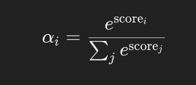
Calculating the exponentials:
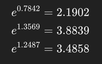
Calculating the sum:

Calculating attention weights:
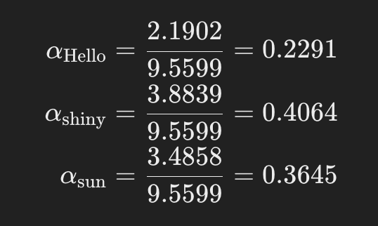
Step 3: Compute the Context Vector
[!TIP] Just get each attention weight and multiply it to the related token dimensions and then sum all the dimensions to get just 1 vector (the context vector)
The context vector is computed as the weighted sum of the embeddings of all words, using the attention weights.

Calculating each component:
- Weighted Embedding of "Hello":

- Weighted Embedding of "shiny":

- Weighted Embedding of "sun":

Summing the weighted embeddings:
context vector=[0.0779+0.2156+0.1057, 0.0504+0.1382+0.1972, 0.1237+0.3983+0.3390]=[0.3992,0.3858,0.8610]
This context vector represents the enriched embedding for the word "shiny," incorporating information from all words in the sentence.
Summary of the Process
- Compute Attention Scores: Use the dot product between the embedding of the target word and the embeddings of all words in the sequence.
- Normalize Scores to Get Attention Weights: Apply the softmax function to the attention scores to obtain weights that sum to 1.
- Compute Context Vector: Multiply each word's embedding by its attention weight and sum the results.
Self-Attention with Trainable Weights
In practice, self-attention mechanisms use trainable weights to learn the best representations for queries, keys, and values. This involves introducing three weight matrices:
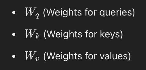
The query is the data to use like before, while the keys and values matrices are just random-trainable matrices.
Step 1: Compute Queries, Keys, and Values
Each token will have its own query, key and value matrix by multiplying its dimension values by the defined matrices:
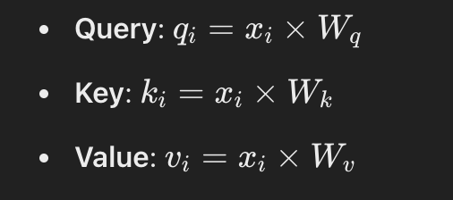
These matrices transform the original embeddings into a new space suitable for computing attention.
Example
Assuming:
- Input dimension
din=3(embedding size) - Output dimension
dout=2(desired dimension for queries, keys, and values)
Initialize the weight matrices:
import torch.nn as nn

d_in = 3
d_out = 2

W_query = nn.Parameter(torch.rand(d_in, d_out))
W_key = nn.Parameter(torch.rand(d_in, d_out))
W_value = nn.Parameter(torch.rand(d_in, d_out))
Compute queries, keys, and values:
queries = torch.matmul(inputs, W_query)
keys = torch.matmul(inputs, W_key)
values = torch.matmul(inputs, W_value)
Step 2: Compute Scaled Dot-Product Attention
Compute Attention Scores
Similar to the example from before, but this time, instead of using the values of the dimensions of the tokens, we use the key matrix of the token (calculated already using the dimensions):. So, for each query qi and key kj:

Scale the Scores
To prevent the dot products from becoming too large, scale them by the square root of the key dimension dk:

[!TIP] The score is divided by the square root of the dimensions because dot products might become very large and this helps to regulate them.
Apply Softmax to Obtain Attention Weights: Like in the initial example, normalize all the values so they sum 1.

Step 3: Compute Context Vectors
Like in the initial example, just sum all the values matrices multiplying each one by its attention weight:

Code Example
Grabbing an example from https://github.com/rasbt/LLMs-from-scratch/blob/main/ch03/01_main-chapter-code/ch03.ipynb you can check this class that implements the self-attendant functionality we talked about:
import torch

inputs = torch.tensor(
  [[0.43, 0.15, 0.89], # Your     (x^1)
   [0.55, 0.87, 0.66], # journey  (x^2)
   [0.57, 0.85, 0.64], # starts   (x^3)
   [0.22, 0.58, 0.33], # with     (x^4)
   [0.77, 0.25, 0.10], # one      (x^5)
   [0.05, 0.80, 0.55]] # step     (x^6)
)

import torch.nn as nn
class SelfAttention_v2(nn.Module):

    def __init__(self, d_in, d_out, qkv_bias=False):
        super().__init__()
        self.W_query = nn.Linear(d_in, d_out, bias=qkv_bias)
        self.W_key   = nn.Linear(d_in, d_out, bias=qkv_bias)
        self.W_value = nn.Linear(d_in, d_out, bias=qkv_bias)

    def forward(self, x):
        keys = self.W_key(x)
        queries = self.W_query(x)
        values = self.W_value(x)

        attn_scores = queries @ keys.T
        attn_weights = torch.softmax(attn_scores / keys.shape[-1]**0.5, dim=-1)

        context_vec = attn_weights @ values
        return context_vec

d_in=3
d_out=2
torch.manual_seed(789)
sa_v2 = SelfAttention_v2(d_in, d_out)
print(sa_v2(inputs))
[!NOTE] Note that instead of initializing the matrices with random values,
nn.Linearis used to mark all the wights as parameters to train.
Causal Attention: Hiding Future Words
For LLMs we want the model to consider only the tokens that appear before the current position in order to predict the next token. Causal attention, also known as masked attention, achieves this by modifying the attention mechanism to prevent access to future tokens.
Applying a Causal Attention Mask
To implement causal attention, we apply a mask to the attention scores before the softmax operation so the reminding ones will still sum 1. This mask sets the attention scores of future tokens to negative infinity, ensuring that after the softmax, their attention weights are zero.
Steps
- Compute Attention Scores: Same as before.
- Apply Mask: Use an upper triangular matrix filled with negative infinity above the diagonal.
mask = torch.triu(torch.ones(seq_len, seq_len), diagonal=1) * float('-inf')
masked_scores = attention_scores + mask
- Apply Softmax: Compute attention weights using the masked scores.
Masking Additional Attention Weights with Dropout
To prevent overfitting, we can apply dropout to the attention weights after the softmax operation. Dropout randomly zeroes some of the attention weights during training.
A regular dropout is about 10-20%.
Code Example
Code example from https://github.com/rasbt/LLMs-from-scratch/blob/main/ch03/01_main-chapter-code/ch03.ipynb:
import torch
import torch.nn as nn

inputs = torch.tensor(
  [[0.43, 0.15, 0.89], # Your     (x^1)
   [0.55, 0.87, 0.66], # journey  (x^2)
   [0.57, 0.85, 0.64], # starts   (x^3)
   [0.22, 0.58, 0.33], # with     (x^4)
   [0.77, 0.25, 0.10], # one      (x^5)
   [0.05, 0.80, 0.55]] # step     (x^6)
)

batch = torch.stack((inputs, inputs), dim=0)
print(batch.shape)

class CausalAttention(nn.Module):

    def __init__(self, d_in, d_out, context_length,
                 dropout, qkv_bias=False):
        super().__init__()
        self.d_out = d_out
        self.W_query = nn.Linear(d_in, d_out, bias=qkv_bias)
        self.W_key   = nn.Linear(d_in, d_out, bias=qkv_bias)
        self.W_value = nn.Linear(d_in, d_out, bias=qkv_bias)
        self.dropout = nn.Dropout(dropout)
        self.register_buffer('mask', torch.triu(torch.ones(context_length, context_length), diagonal=1)) # New

    def forward(self, x):
        b, num_tokens, d_in = x.shape
        # b is the num of batches
        # num_tokens is the number of tokens per batch
        # d_in is the dimensions er token

        keys = self.W_key(x) # This generates the keys of the tokens
        queries = self.W_query(x)
        values = self.W_value(x)

        attn_scores = queries @ keys.transpose(1, 2) # Moves the third dimension to the second one and the second one to the third one to be able to multiply
        attn_scores.masked_fill_(  # New, _ ops are in-place
            self.mask.bool()[:num_tokens, :num_tokens], -torch.inf)  # `:num_tokens` to account for cases where the number of tokens in the batch is smaller than the supported context_size
        attn_weights = torch.softmax(
            attn_scores / keys.shape[-1]**0.5, dim=-1
        )
        attn_weights = self.dropout(attn_weights)

        context_vec = attn_weights @ values
        return context_vec

torch.manual_seed(123)

context_length = batch.shape[1]
d_in = 3
d_out = 2
ca = CausalAttention(d_in, d_out, context_length, 0.0)

context_vecs = ca(batch)

print(context_vecs)
print("context_vecs.shape:", context_vecs.shape)
Extending Single-Head Attention to Multi-Head Attention
Multi-head attention in practical terms consist on executing multiple instances of the self-attention function each of them with their own weights so different final vectors are calculated.
Code Example
It could be possible to reuse the previous code and just add a wrapper that launches it several time, but this is a more optimised version from https://github.com/rasbt/LLMs-from-scratch/blob/main/ch03/01_main-chapter-code/ch03.ipynb that processes all the heads at the same time (reducing the number of expensive for loops). As you can see in the code, the dimensions of each token is divided in different dimensions according to the number of heads. This way if token have 8 dimensions and we want to use 3 heads, the dimensions will be divided in 2 arrays of 4 dimensions and each head will use one of them:
class MultiHeadAttention(nn.Module):
    def __init__(self, d_in, d_out, context_length, dropout, num_heads, qkv_bias=False):
        super().__init__()
        assert (d_out % num_heads == 0), \
            "d_out must be divisible by num_heads"

        self.d_out = d_out
        self.num_heads = num_heads
        self.head_dim = d_out // num_heads # Reduce the projection dim to match desired output dim

        self.W_query = nn.Linear(d_in, d_out, bias=qkv_bias)
        self.W_key = nn.Linear(d_in, d_out, bias=qkv_bias)
        self.W_value = nn.Linear(d_in, d_out, bias=qkv_bias)
        self.out_proj = nn.Linear(d_out, d_out)  # Linear layer to combine head outputs
        self.dropout = nn.Dropout(dropout)
        self.register_buffer(
            "mask",
            torch.triu(torch.ones(context_length, context_length),
                       diagonal=1)
        )

    def forward(self, x):
        b, num_tokens, d_in = x.shape
        # b is the num of batches
        # num_tokens is the number of tokens per batch
        # d_in is the dimensions er token

        keys = self.W_key(x) # Shape: (b, num_tokens, d_out)
        queries = self.W_query(x)
        values = self.W_value(x)

        # We implicitly split the matrix by adding a `num_heads` dimension
        # Unroll last dim: (b, num_tokens, d_out) -> (b, num_tokens, num_heads, head_dim)
        keys = keys.view(b, num_tokens, self.num_heads, self.head_dim)
        values = values.view(b, num_tokens, self.num_heads, self.head_dim)
        queries = queries.view(b, num_tokens, self.num_heads, self.head_dim)

        # Transpose: (b, num_tokens, num_heads, head_dim) -> (b, num_heads, num_tokens, head_dim)
        keys = keys.transpose(1, 2)
        queries = queries.transpose(1, 2)
        values = values.transpose(1, 2)

        # Compute scaled dot-product attention (aka self-attention) with a causal mask
        attn_scores = queries @ keys.transpose(2, 3)  # Dot product for each head

        # Original mask truncated to the number of tokens and converted to boolean
        mask_bool = self.mask.bool()[:num_tokens, :num_tokens]

        # Use the mask to fill attention scores
        attn_scores.masked_fill_(mask_bool, -torch.inf)

        attn_weights = torch.softmax(attn_scores / keys.shape[-1]**0.5, dim=-1)
        attn_weights = self.dropout(attn_weights)

        # Shape: (b, num_tokens, num_heads, head_dim)
        context_vec = (attn_weights @ values).transpose(1, 2)

        # Combine heads, where self.d_out = self.num_heads * self.head_dim
        context_vec = context_vec.contiguous().view(b, num_tokens, self.d_out)
        context_vec = self.out_proj(context_vec) # optional projection

        return context_vec

torch.manual_seed(123)

batch_size, context_length, d_in = batch.shape
d_out = 2
mha = MultiHeadAttention(d_in, d_out, context_length, 0.0, num_heads=2)

context_vecs = mha(batch)

print(context_vecs)
print("context_vecs.shape:", context_vecs.shape)
For another compact and efficient implementation you could use the torch.nn.MultiheadAttention class in PyTorch.
[!TIP] Short answer of ChatGPT about why it's better to divide dimensions of tokens among the heads instead of having each head check all the dimensions of all the tokens:
While allowing each head to process all embedding dimensions might seem advantageous because each head would have access to the full information, the standard practice is to divide the embedding dimensions among the heads. This approach balances computational efficiency with model performance and encourages each head to learn diverse representations. Therefore, splitting the embedding dimensions is generally preferred over having each head check all dimensions.