0. Basic LLM Concepts
Pretraining
Pretraining is the foundational phase in developing a large language model (LLM) where the model is exposed to vast and diverse amounts of text data. During this stage, the LLM learns the fundamental structures, patterns, and nuances of language, including grammar, vocabulary, syntax, and contextual relationships. By processing this extensive data, the model acquires a broad understanding of language and general world knowledge. This comprehensive base enables the LLM to generate coherent and contextually relevant text. Subsequently, this pretrained model can undergo fine-tuning, where it is further trained on specialized datasets to adapt its capabilities for specific tasks or domains, enhancing its performance and relevance in targeted applications.
Main LLM components
Usually a LLM is characterised for the configuration used to train it. This are the common components when training a LLM:
- Parameters: Parameters are the learnable weights and biases in the neural network. These are the numbers that the training process adjusts to minimize the loss function and improve the model's performance on the task. LLMs usually use millions of parameters.
- Context Length: This is the maximum length of each sentence used to pre-train the LLM.
- Embedding Dimension: The size of the vector used to represent each token or word. LLMs usually sue billions of dimensions.
- Hidden Dimension: The size of the hidden layers in the neural network.
- Number of Layers (Depth): How many layers the model has. LLMs usually use tens of layers.
- Number of Attention Heads: In transformer models, this is how many separate attention mechanisms are used in each layer. LLMs usually use tens of heads.
- Dropout: Dropout is something like the percentage of data that is removed (probabilities turn to 0) during training used to prevent overfitting. LLMs usually use between 0-20%.
Configuration of the GPT-2 model:
GPT_CONFIG_124M = {
    "vocab_size": 50257,  // Vocabulary size of the BPE tokenizer
    "context_length": 1024, // Context length
    "emb_dim": 768,       // Embedding dimension
    "n_heads": 12,        // Number of attention heads
    "n_layers": 12,       // Number of layers
    "drop_rate": 0.1,     // Dropout rate: 10%
    "qkv_bias": False     // Query-Key-Value bias
}
Tensors in PyTorch
In PyTorch, a tensor is a fundamental data structure that serves as a multi-dimensional array, generalizing concepts like scalars, vectors, and matrices to potentially higher dimensions. Tensors are the primary way data is represented and manipulated in PyTorch, especially in the context of deep learning and neural networks.
Mathematical Concept of Tensors
- Scalars: Tensors of rank 0, representing a single number (zero-dimensional). Like: 5
- Vectors: Tensors of rank 1, representing a one-dimensional array of numbers. Like: [5,1]
- Matrices: Tensors of rank 2, representing two-dimensional arrays with rows and columns. Like: [[1,3], [5,2]]
- Higher-Rank Tensors: Tensors of rank 3 or more, representing data in higher dimensions (e.g., 3D tensors for color images).
Tensors as Data Containers
From a computational perspective, tensors act as containers for multi-dimensional data, where each dimension can represent different features or aspects of the data. This makes tensors highly suitable for handling complex datasets in machine learning tasks.
PyTorch Tensors vs. NumPy Arrays
While PyTorch tensors are similar to NumPy arrays in their ability to store and manipulate numerical data, they offer additional functionalities crucial for deep learning:
- Automatic Differentiation: PyTorch tensors support automatic calculation of gradients (autograd), which simplifies the process of computing derivatives required for training neural networks.
- GPU Acceleration: Tensors in PyTorch can be moved to and computed on GPUs, significantly speeding up large-scale computations.
Creating Tensors in PyTorch
You can create tensors using the torch.tensor function:
pythonCopy codeimport torch

# Scalar (0D tensor)
tensor0d = torch.tensor(1)

# Vector (1D tensor)
tensor1d = torch.tensor([1, 2, 3])

# Matrix (2D tensor)
tensor2d = torch.tensor([[1, 2],
                         [3, 4]])

# 3D Tensor
tensor3d = torch.tensor([[[1, 2], [3, 4]],
                         [[5, 6], [7, 8]]])
Tensor Data Types
PyTorch tensors can store data of various types, such as integers and floating-point numbers.
You can check a tensor's data type using the .dtype attribute:
- Tensors created from Python integers are of type
torch.int64. - Tensors created from Python floats are of type
torch.float32.
To change a tensor's data type, use the .to() method:
Common Tensor Operations
PyTorch provides a variety of operations to manipulate tensors:
- Accessing Shape: Use
.shapeto get the dimensions of a tensor.
- Reshaping Tensors: Use
.reshape()or.view()to change the shape.
- Transposing Tensors: Use
.Tto transpose a 2D tensor.
- Matrix Multiplication: Use
.matmul()or the@operator.
Importance in Deep Learning
Tensors are essential in PyTorch for building and training neural networks:
- They store input data, weights, and biases.
- They facilitate operations required for forward and backward passes in training algorithms.
- With autograd, tensors enable automatic computation of gradients, streamlining the optimization process.
Automatic Differentiation
Automatic differentiation (AD) is a computational technique used to evaluate the derivatives (gradients) of functions efficiently and accurately. In the context of neural networks, AD enables the calculation of gradients required for optimization algorithms like gradient descent. PyTorch provides an automatic differentiation engine called autograd that simplifies this process.
Mathematical Explanation of Automatic Differentiation
1. The Chain Rule
At the heart of automatic differentiation is the chain rule from calculus. The chain rule states that if you have a composition of functions, the derivative of the composite function is the product of the derivatives of the composed functions.
Mathematically, if y=f(u) and u=g(x), then the derivative of y with respect to x is:

2. Computational Graph
In AD, computations are represented as nodes in a computational graph, where each node corresponds to an operation or a variable. By traversing this graph, we can compute derivatives efficiently.
- Example
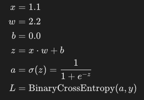
Let's consider a simple function:

Where:
σ(z)is the sigmoid function.y=1.0is the target label.Lis the loss.
We want to compute the gradient of the loss L with respect to the weight w and bias b.
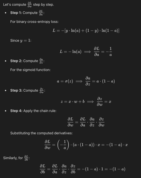
4. Computing Gradients Manually

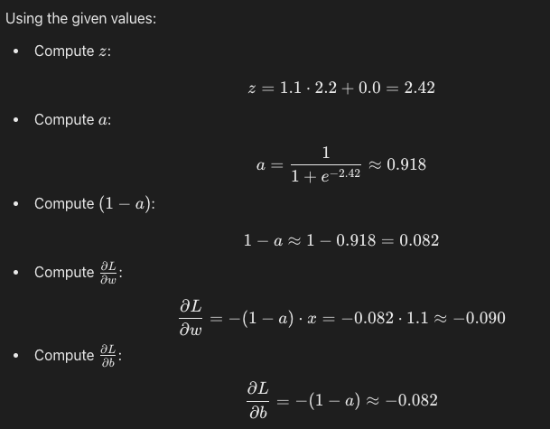
5. Numerical Calculation

Implementing Automatic Differentiation in PyTorch
Now, let's see how PyTorch automates this process.
pythonCopy codeimport torch
import torch.nn.functional as F

# Define input and target
x = torch.tensor([1.1])
y = torch.tensor([1.0])

# Initialize weights with requires_grad=True to track computations
w = torch.tensor([2.2], requires_grad=True)
b = torch.tensor([0.0], requires_grad=True)

# Forward pass
z = x * w + b
a = torch.sigmoid(z)
loss = F.binary_cross_entropy(a, y)

# Backward pass
loss.backward()

# Gradients
print("Gradient w.r.t w:", w.grad)
print("Gradient w.r.t b:", b.grad)
Output:
Backpropagation in Bigger Neural Networks
1.Extending to Multilayer Networks
In larger neural networks with multiple layers, the process of computing gradients becomes more complex due to the increased number of parameters and operations. However, the fundamental principles remain the same:
- Forward Pass: Compute the output of the network by passing inputs through each layer.
- Compute Loss: Evaluate the loss function using the network's output and the target labels.
- Backward Pass (Backpropagation): Compute the gradients of the loss with respect to each parameter in the network by applying the chain rule recursively from the output layer back to the input layer.
2. Backpropagation Algorithm
- Step 1: Initialize the network parameters (weights and biases).
- Step 2: For each training example, perform a forward pass to compute the outputs.
- Step 3: Compute the loss.
- Step 4: Compute the gradients of the loss with respect to each parameter using the chain rule.
- Step 5: Update the parameters using an optimization algorithm (e.g., gradient descent).
3. Mathematical Representation
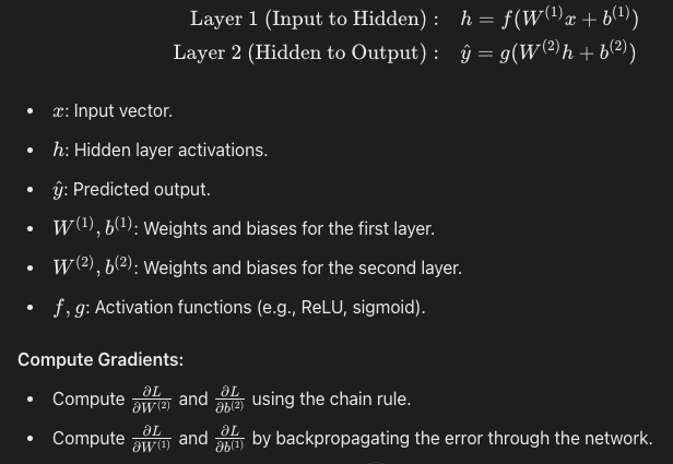
Consider a simple neural network with one hidden layer:

4. PyTorch Implementation
PyTorch simplifies this process with its autograd engine.
import torch
import torch.nn as nn
import torch.optim as optim

# Define a simple neural network
class SimpleNet(nn.Module):
    def __init__(self):
        super(SimpleNet, self).__init__()
        self.fc1 = nn.Linear(10, 5)  # Input layer to hidden layer
        self.relu = nn.ReLU()
        self.fc2 = nn.Linear(5, 1)   # Hidden layer to output layer
        self.sigmoid = nn.Sigmoid()

    def forward(self, x):
        h = self.relu(self.fc1(x))
        y_hat = self.sigmoid(self.fc2(h))
        return y_hat

# Instantiate the network
net = SimpleNet()

# Define loss function and optimizer
criterion = nn.BCELoss()
optimizer = optim.SGD(net.parameters(), lr=0.01)

# Sample data
inputs = torch.randn(1, 10)
labels = torch.tensor([1.0])

# Training loop
optimizer.zero_grad()          # Clear gradients
outputs = net(inputs)          # Forward pass
loss = criterion(outputs, labels)  # Compute loss
loss.backward()                # Backward pass (compute gradients)
optimizer.step()               # Update parameters

# Accessing gradients
for name, param in net.named_parameters():
    if param.requires_grad:
        print(f"Gradient of {name}: {param.grad}")
In this code:
- Forward Pass: Computes the outputs of the network.
- Backward Pass:
loss.backward()computes the gradients of the loss with respect to all parameters. - Parameter Update:
optimizer.step()updates the parameters based on the computed gradients.
5. Understanding Backward Pass
During the backward pass:
- PyTorch traverses the computational graph in reverse order.
- For each operation, it applies the chain rule to compute gradients.
- Gradients are accumulated in the
.gradattribute of each parameter tensor.
6. Advantages of Automatic Differentiation
- Efficiency: Avoids redundant calculations by reusing intermediate results.
- Accuracy: Provides exact derivatives up to machine precision.
- Ease of Use: Eliminates manual computation of derivatives.